- Note
- The example is based on Litvinenko, Sun, Genton and Keyes, Likelihood Approximation With H-Matrices For Large Spatial Datasets (arXiv:1709.04419).
Problem Description
The number of measurements that must be processed for statistical modeling in environmental applications is usually very large, and these measurements may be located irregularly across a given geographical region. This makes the computing process expensive and the data difficult to manage.
These data are frequently modeled as a realization from a stationary Gaussian spatial random field. Specifically, we let \(\mathbf{Z}=\{Z(\mathbf{s}_1),\ldots,Z(\mathbf{s}_n)\}^\top\), where \(Z(\mathbf{s})\) is a Gaussian random field indexed by a spatial location \(\mathbf{s} \in \Bbb{R}^d\), \(d\geq 1\). Then, we assume that \(\mathbf{Z}\) has mean zero and a stationary parametric covariance function
\[ C(\mathbf{h};{\boldsymbol \theta})=\hbox{cov}\{Z(\mathbf{s}),Z(\mathbf{s}+\mathbf{h})\}, \]
where \(\mathbf{h}\in\Bbb{R}^d\) is a spatial lag vector and \({\boldsymbol \theta}\in\Bbb{R}^q\) is the unknown parameter vector of interest. Statistical inferences about \({\boldsymbol \theta}\) are often based on the joint Gaussian log-likelihood function:
\[ \mathcal{L}(\mathbf{\theta})=-\frac{n}{2}\log(2\pi) - \frac{1}{2}\log \vert \mathbf{C}(\mathbf{\theta}) \vert-\frac{1}{2}\mathbf{Z}^\top \mathbf{C}(\mathbf{\theta})^{-1}\mathbf{Z}, \]
where the covariance matrix \(\mathbf{C}(\mathbf{\theta})\) has entries \(C(\mathbf{s}_i-\mathbf{s}_j;{\boldsymbol \theta})\), \(i,j=1,\ldots,n\). The maximum likelihood estimator of \({\boldsymbol \theta}\) is the value \(\widehat{\boldsymbol \theta}\) that maximizes \(\mathcal{L}\). When the sample size \(n\) is large, the evaluation of \(\mathcal{L}\) becomes challenging, due to the computation of the inverse and log-determinant of the \(n\)-by- \(n\) covariance matrix \(\mathbf{C}(\mathbf{\theta})\). Indeed, this requires \({\cal O}(n^2)\) memory and \({\cal O}(n^3)\) computational steps. Hence, scalable methods that can process larger sample sizes are needed which in this example are provided by \(\mathcal{H}\)-matrices and their arithmetic.
Matérn Covariance Function
Among the many covariance models available, the Matérn family has gained widespread interest in recent years. The Matérn form of spatial correlations was introduced into statistics as a flexible parametric class, with one parameter determining the smoothness of the underlying spatial random field.
The Matérn covariance depends only on the distance \(h:=\Vert \mathbf{s}-\mathbf{s}'\Vert \), where \(\mathbf{s}\) and \(\mathbf{s}'\) are any two spatial locations. The Matérn class of covariance functions is defined as
\[ C(h;{\boldsymbol\theta})=\frac{\sigma^2}{2^{\nu-1}\Gamma(\nu)}\left(\frac{h}{\ell}\right)^\nu K_\nu\left(\frac{h}{\ell}\right), \]
with \({\boldsymbol\theta}=(\sigma^2,\ell,\nu)^\top\); where \(\sigma^2\) is the variance; \(\nu>0\) controls the smoothness of the random field, with larger values of \(\nu\) corresponding to smoother fields; and \(\ell>0\) is a spatial range parameter that measures how quickly the correlation of the random field decays with distance, with larger \(\ell\) corresponding to a faster decay (keeping \(\nu\) fixed). Here \({\mathcal{K}}_\nu\) denotes the modified Bessel function of the second kind of order \(\nu\). When \(\nu=1/2\), the Matérn covariance function reduces to the exponential covariance model and describes a rough field. The value \(\nu=\infty\) corresponds to a Gaussian covariance model that describes a very smooth, infinitely differentiable field. Random fields with a Matérn covariance function are \(\lfloor \nu-1 \rfloor\) times mean square differentiable.
Hierarchical Approximation of Gaussian Log-Likelihood
We use the \(\mathcal{H}\)-matrix technique to approximate the Gaussian likelihood function. The \(\mathcal{H}\)-matrix approximation of the exact log-likelihood \(\mathcal{L}({\boldsymbol\theta})\) is defined by \(\tilde{\mathcal{L}}({\boldsymbol\theta})\):
\[ \tilde{\mathcal{L}}({\boldsymbol\theta})=-\frac{n}{2}\log(2\pi) - \sum_{i=1}^n\log \{\tilde{\mathbf{L}}_{ii}({\boldsymbol\theta})\}-\frac{1}{2}\mathbf{v}({\boldsymbol\theta})^\top \mathbf{v}({\boldsymbol\theta}), \]
where \(\tilde{\mathbf{L}}({\boldsymbol\theta})\) is the \(\mathcal{H}\)-matrix approximation of the Cholesky factor \(\mathbf{L}({\boldsymbol\theta})\) in \(\mathbf{C}({\boldsymbol\theta})=\mathbf{L}({\boldsymbol\theta})\mathbf{L}({\boldsymbol\theta})^\top\), and \(\mathbf{v}({\boldsymbol\theta}) \) is the solution of the linear system \(\tilde{\mathbf{L}}({\boldsymbol\theta})\mathbf{v}({\boldsymbol\theta})=\mathbf{Z}\).
Since the representation of the dense \(\boldsymbol C(\theta)\) requires quadratic storage complexity, approximation is already applied here, e.g., \(\tilde C(\theta)\) is computed instead as an \(\mathcal{H}\)-matrix approximation of \(\boldsymbol C(\theta)\). With this, we obtain \(\tilde{\mathbf{L}}({\boldsymbol\theta})\) as the Cholesky factor in the factorization
\[ \mathbf{\tilde C}({\boldsymbol\theta})=\mathbf{\tilde L}({\boldsymbol\theta})\mathbf{\tilde L}({\boldsymbol\theta})^\top \]
For the \(\mathcal{H}\)-matrix approximation \(\tilde{\mathcal{L}}({\boldsymbol\theta})\) we can either choose a constant rank \(k\), e.g., all low-rank subblocks of the matrix are of rank \(k\), or a fixed accuracy \(\varepsilon > 0\). In the latter case, the rank per subblock is adaptively chosen (see also Accuracy Control).
Of further interest is the value \(\hat \theta\) which maximizes \(\mathcal{L}(\theta)\), which is a three dimensional optimization problem for \((\sigma^2,\ell,\nu)\).
Implementation
The program starts with the usual inclusion of the corresponding HLIBpro header files and the initialisation of HLIBpro:
#include <iostream>
#include <fstream>
#include <string>
#include <vector>
#include "hlib.hh"
using namespace HLIB;
int
main ( int argc,
char ** argv )
{
INIT();
In the next step, the coordinate and the rhs data is read from a file:
std::vector< T2Point > vertices;
BLAS::Vector< double > Z_data;
size_t N = 0;
read_data( "datafile.txt", vertices, Z_data );
N = vertices.size();
TCoordinate coord( vertices );
The function read_data implements the most part. For the actual data file, a text format is assumed in which in the first line the number of coordinates is given. Afterwards, each line contains the coordinate index (counting starts from zero) followed by two spatial coordinates and the value of \(\boldsymbol Z\) is given.
As an example, the following data defines four values of \(\boldsymbol Z\) at the eight points of a unit cube:
8
0 0 0 0 0.1
0 0 0 1 0.2
0 0 1 0 0.3
0 0 1 1 0.4
0 1 0 0 0.5
0 1 0 1 0.6
0 1 1 0 0.7
0 1 1 1 0.8
The function then looks like:
void
read_data ( const std::string & datafile,
std::vector< T2Point > & vertices,
BLAS::Vector< double > & Z_data )
{
std::ifstream in( datafile );
if ( ! in )
exit( 1 );
size_t N = 0;
in >> N;
vertices.resize( N );
Z_data = BLAS::Vector< double >( N );
for ( idx_t i = 0; i < idx_t(N); ++i )
{
int index = i;
double x, y;
double v = 0.0;
in >> index >> x >> y >> v;
vertices[ index ] = T2Point( x, y );
Z_data( index ) = v;
}
}
Construction of Covariance Matrix
Before the \(\mathcal{H}\)-matrix can be constructed, the block layout of the matrix has to be defined. For this, the coordinates are used to partition the index set. Together with an admissibility condition, the partitioning of the \(\mathcal{H}\)-matrix is defined:
TAutoBSPPartStrat part_strat;
TBSPCTBuilder ct_builder( & part_strat );
auto ct = ct_builder.build( & coord );
TStdGeomAdmCond adm_cond( 2.0 );
TBCBuilder bct_builder;
auto bct = bct_builder.build( ct.get(), ct.get(), & adm_cond );
For the \(\mathcal{H}\)-matrix, the matrix coefficients have to be computed. HLIBpro provides the Matern coefficient function in the form of TMaternCovCoeffFn, which expects a template argument to define the type in which coordinates are provided. In this example, this corresponds to T2DPoint for two dimensional coordinates.
Furthermore, the parameters \(\sigma, \ell\) and \(\nu\) need to be defined. For now, we assume some fixed values for these (see below for maximization of covariance function):
const double sigma = 1.0;
const double length = 9.0e-2;
const double nu = 0.5;
With this, the coefficient function for the Matern kernel can be defined:
TMaternCovCoeffFn< T2Point > matern_coefffn( sigma, length, nu, vertices );
TPermCoeffFn< double > coefffn( & matern_coefffn, ct->perm_i2e(), ct->perm_i2e() );
The permutation function converts the numbering from the numberung due to the coordinate indices to the internal numbering of the \(\mathcal{H}\)-matrix.
Equipped with matrix coefficients, we finally can construct the \(\mathcal{H}\)-matrix approximation to \(\boldsymbol C(\theta)\):
TACAPlus< double > aca( & coefffn );
double eps = 1e-4;
auto acc = fixed_prec( eps );
TDenseMatBuilder< double > h_builder( & coefffn, & aca );
auto C = h_builder.build( bct.get(), acc );
Computation of Log-Determinant
First, the cholesky factorization needs to be computed of C:
auto C_fac = C->copy();
chol( C_fac.get(), acc );
auto C_inv = std::make_unique< TLLInvMatrix >( C_fac.get(), symmetric );
At this point, C_inv is a linear operator enabling evaluation of \(C^{-1}\) while C_fac holds the entries of the Cholesky factor.
The latter are now of interest as we need to compute the log-determinant. Since \(\tilde L\) is of triangular shape and after switching multiplication with logarithm, a summation of the logarithm of its diagonal elements yields the result:
double log_det_C = 0.0;
for ( idx_t i = 0; i < idx_t(N); ++i )
log_det_C += 2*std::log( C_fac->entry( i, i ) );
Computation of Gaussian Log-Likelihood
Finally, we are able to compute the Gaussian log-likelihood \(\mathcal{L}(\theta)\). Only missing is the vector \(v(\theta)\) as the solution of the rhs \(Z\) and the covariance matrix \(C\).
First, the right hand side is set up with the previously read data:
auto Z = std::make_unique< TScalarVector >( *ct->root(), Z_data );
ct->perm_e2i()->permute( Z.get() );
The last step is necessary for the vector to have the same ordering as the \(\mathcal{H}\)-matrix.
Solving the equation system is done iteratively using the Cholesky factorization as a preconditioner.
TStopCriterion sstop( 250, 1e-16, 0.0 );
TCG solver( sstop );
auto sol = C->row_vector();
solver.solve( C.get(), sol.get(), Z.get(), C_inv.get() );
The stop criterion was chosen to have at most 250 iterations and to reduce the residual by a factor of \(10^{16}\). The CG solver is used since \(C\) is positive definite.
After iteration sol holds the solution.
The log-likelihood LL is then computed following the above formula as
auto ZdotCZ = std::real( Z->dot( sol.get() ) );
const double log2pi = std::log( 2.0 * Math::pi<double>() );
auto LL = -0.5 * ( N * log2pi + log_det_C + ZdotCZ );
std::cout << " " << "LogLi = " << LL << std::endl;
With the finalization of HLIBpro
the program for computing the log-likelihood for a fixed parameter set \(\theta\) is complete.
Example Data
Example data for the program is provided by a soil moisture data set with 4000 data points and corresponding values of \(Z\).
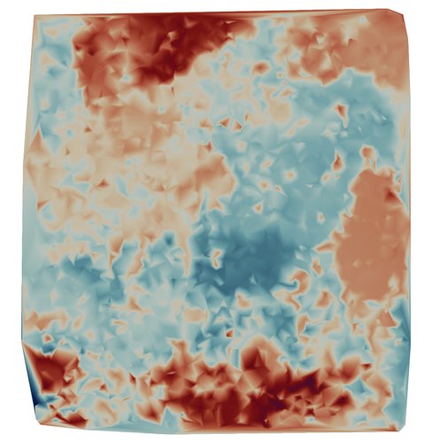 |
| Example Moisture Data |
You may download the data file from hlibpro.com.
Vizualization
The data assigns a parameter to each spatial point. The program ParaView is able to visualize this point data. For this, we write the coordinates and the parameter in a CSV (comma separated) file:
void
write_csv ( const std::string & csvfile,
const std::vector< T2Point > & vertices,
const BLAS::Vector< double > & Z_data )
{
std::ofstream out( csvfile );
out << "x,y,z,v" << std::endl;
for ( uint i = 0; i < vertices.size(); ++i )
out << vertices[i].x() << "," << vertices[i].y() << ",0," << Z_data( i ) << std::endl;
}
In ParaView, open the CSV file and press Apply. The default options for importing CSV data work with the format of the above export function.
After importing, the data is shown as a table. This table is now converted to point data by choosing Filter > Alphabetical > Table to Points. Choose x for the X column, y for the Y column and z for the Z column. You may also activate 2D Points as the data is two dimensional (z set to zero). After pressing Apply, the points should be visible in the Render View. If not, make sure the eye symbol next to TableToPoints1 is active.
Afterwards, you may use the v values for colorization of the points. Just select in the left pane at Coloring v instead of Solid Color (you may also change the colormap).
ParaView also lets you convert the point cloud into a grid. For this, use Filters > Alphabetical > Delaunay 2D and press Apply.
Modifications
LDL factorization
Instead of using the Cholesky factorization to compute the log-determinant and the preconditioner for solving \(C(\theta) v = Z\), one could use LDL factorization which is more stable in case of rounding errors leading to negative diagonal elements during Cholesky (the covariance matrix becomes ill-conditioned with a larger problem dimension).
By default, HLIBpro computes a block-wise LDL factorization, e.g., computing the inverse of diagonal block instead of performing dense LDL. Since the diagonal elements of \(D\) are needed, this is not possible. Therefore, the point-wise version needs to be performed, which is enabled by setting the corresponding option before factorization:
fac_options_t fac_options;
fac_options.eval = point_wise;
ldl( C_fac.get(), acc, fac_options );
C_inv = std::make_unique< TLDLInvMatrix >( C_fac.get(), symmetric, point_wise );
void ldl(TMatrix *A, const TTruncAcc &acc, const fac_options_t &options=fac_options_t())
compute LDL^H factorisation
The computation of the log-determinant also changes, since now only \(D\) has to be considered with \(L\) being unit diagonal matrices:
for ( idx_t i = 0; i < idx_t(N); ++i )
log_det_C += std::log( C_fac->entry( i, i ) );
Three Dimensional Data
As the implementation of the Matern kernel is based on a template argument for the coordinates, it is easy to modify the code to support three dimensional data: just replace T2Point with T3Point. Furthermore, you have to read the third coordinate in read_data:
void
read_data ( const string & datafile,
std::vector< T3Point > & vertices,
BLAS::Vector< double > & Z_data )
{
std::ifstream in( datafile );
if ( ! in )
exit( 1 );
size_t N = 0;
in >> N;
vertices.resize( N );
Z_data = BLAS::Vector< double >( N );
for ( idx_t i = 0; i < idx_t(N); ++i )
{
int index = i;
double x, y, z;
double v = 0.0;
in >> index >> x >> y >> z >> v;
vertices[ index ] = T3Point( x, y, z );
Z_data( index ) = v;
}
}
The Plain Program
#include <iostream>
#include <fstream>
#include <string>
#include <vector>
#include "hlib.hh"
using namespace HLIB;
void
read_data ( const std::string & datafile,
std::vector< T2Point > & vertices,
BLAS::Vector< double > & Z_data )
{
std::ifstream in( datafile );
if ( ! in )
exit( 1 );
size_t N = 0;
in >> N;
vertices.resize( N );
Z_data = BLAS::Vector< double >( N );
for ( idx_t i = 0; i < idx_t(N); ++i )
{
int index = i;
double x, y;
double v = 0.0;
in >> index >> x >> y >> v;
vertices[ index ] = T2Point( x, y );
Z_data( index ) = v;
}
}
int
main ( int argc,
char ** argv )
{
INIT();
std::vector< T2Point > vertices;
BLAS::Vector< double > Z_data;
size_t N = 0;
read_data( "datafile.txt", vertices, Z_data );
N = vertices.size();
TCoordinate coord( vertices );
TAutoBSPPartStrat part_strat;
TBSPCTBuilder ct_builder( & part_strat );
auto ct = ct_builder.build( & coord );
TStdGeomAdmCond adm_cond( 2.0 );
TBCBuilder bct_builder;
auto bct = bct_builder.build( ct.get(), ct.get(), & adm_cond );
const double sigma = 1.0;
const double length = 9.0e-2;
const double nu = 0.5;
TMaternCovCoeffFn< T2Point > matern_coefffn( sigma, length, nu, vertices );
TPermCoeffFn< double > coefffn( & matern_coefffn, ct->perm_i2e(), ct->perm_i2e() );
TACAPlus< double > aca( & coefffn );
double eps = 1e-4;
auto acc = fixed_prec( eps );
TDenseMatBuilder< double > h_builder( & coefffn, & aca );
auto C = h_builder.build( bct.get(), acc );
auto C_fac = C->copy();
chol( C_fac.get(), acc );
auto C_inv = std::make_unique< TLLInvMatrix >( C_fac.get(), symmetric );
double log_det_C = 0.0;
for ( idx_t i = 0; i < idx_t(N); ++i )
log_det_C += 2*std::log( C_fac->entry( i, i ) );
auto Z = std::make_unique< TScalarVector >( *ct->root(), Z_data );
ct->perm_e2i()->permute( Z.get() );
TStopCriterion sstop( 250, 1e-16, 0.0 );
TCG solver( sstop );
auto sol = C->row_vector();
solver.solve( C.get(), sol.get(), Z.get(), C_inv.get() );
auto ZdotCZ = std::real( Z->dot( sol.get() ) );
const double log2pi = std::log( 2.0 * Math::pi<double>() );
auto LL = -0.5 * ( N * log2pi + log_det_C + ZdotCZ );
std::cout << " " << "LogLi = " << LL << std::endl;
DONE();
return 0;
}
Maximization of Log-Likelihood
Function Minimization
The GNU Scientific Library is used to implement the maximization of \(\mathcal{L}(\theta)\) by corresponding minimization functions provided by GSL and we wrap the process into a corresponding function:
#include <gsl/gsl_multimin.h>
enum {
IDX_SIGMA = 0,
IDX_LENGTH = 1,
IDX_NU = 2
};
double
maximize_likelihood ( double & sigma,
double & length,
double & nu,
LogLikeliHoodProblem & problem )
{
The first three parameters provide the start value for the maximization on input and hold the maximal values on output of the function. The last parameter, which corresponds to the problem to maximize is discussed below.
First, the GSL data structures are intialized with the start value and step sizes for each parameter. Since the parameters are entries in an array, we use the above predefined indices to access those.
int status = 0;
const int max_iter = 200;
const gsl_multimin_fminimizer_type * T = gsl_multimin_fminimizer_nmsimplex2;
gsl_multimin_fminimizer * s = NULL;
gsl_vector * ss;
gsl_vector * x;
gsl_multimin_function minex_func;
double size;
x = gsl_vector_alloc( 3 );
gsl_vector_set( x, 0, sigma );
gsl_vector_set( x, 1, length );
gsl_vector_set( x, 2, nu );
ss = gsl_vector_alloc( 3 );
gsl_vector_set( ss, IDX_SIGMA, 0.001 );
gsl_vector_set( ss, IDX_LENGTH, 0.004 );
gsl_vector_set( ss, IDX_NU, 0.002 );
Next, the function to maximize (minimize) is defined.
minex_func.n = 3;
minex_func.f = & eval_logli;
minex_func.params = & problem;
Here, eval_logli implements the evaluation of the Gaussian log-likelihood for a given parameter \(\theta = (\sigma,\ell,\nu)\). The second parameter to this function is set to the problem object and cast back inside to be evaluated.
The return value of eval is negated, because GSL performs a function minimization instead of maximization.
double
eval_logli ( const gsl_vector * param,
void * data )
{
double sigma = gsl_vector_get( param, IDX_SIGMA );
double length = gsl_vector_get( param, IDX_LENGTH );
double nu = gsl_vector_get( param, IDX_NU );
LogLikeliHoodProblem * problem = static_cast< LogLikeliHoodProblem * >( data );
return - problem->eval( sigma, length, nu );
}
The GSL part is continued with setting up the iterative s and starting the actual minimization loop:
s = gsl_multimin_fminimizer_alloc( T, 3 );
gsl_multimin_fminimizer_set(s, & minex_func, x, ss );
int iter = 0;
double LL = 0;
do
{
iter++;
Next, a single minimization step is performed and the accuracy criterion tested (tolerance \(\le 10^{-3}\)):
status = gsl_multimin_fminimizer_iterate( s );
if ( status != 0 )
break;
size = gsl_multimin_fminimizer_size( s );
status = gsl_multimin_test_size( size, 1e-3 );
if ( status == GSL_SUCCESS )
std::cout << "converged to minimum" << std::endl;
The individual parameters are extracted together with the value of the log-likelihood for the current value of \(\theta\):
sigma = gsl_vector_get( s->x, IDX_SIGMA );
length = gsl_vector_get( s->x, IDX_LENGTH );
nu = gsl_vector_get( s->x, IDX_NU );
LL = -s->fval;
Stop the iteration if the accuracy tolerance was achieved or the maximal number of iterations reached.
} while (( status == GSL_CONTINUE ) && ( iter < max_iter ));
gsl_multimin_fminimizer_free( s );
gsl_vector_free( ss );
gsl_vector_free( x );
return LL;
}
Log-Likelihood Problem
Above, the Gaussian log-likelihood problem was evaluated for a fixed parameter \(\theta\). Now, we need to evaluate this for many different values and hence, we restructure the code, which splits constant parts, e.g. coordinate managment and partitioning, and variable parts, e.g., \(\mathcal{H}\)-matrix approximation and factorization, into different functions.
struct LogLikeliHoodProblem
{
std::vector< T2Point > vertices;
std::unique_ptr< TCoordinate > coord;
std::unique_ptr< TClusterTree > ct;
std::unique_ptr< TBlockClusterTree > bct;
std::unique_ptr< TVector > Z;
double eps;
LogLikeliHoodProblem ( const std::string & coord_filename,
const double accuracy )
: eps( accuracy )
{
init( coord_filename );
}
void
init ( const std::string & datafile );
double
eval (
const double sigma,
const double length,
const double nu );
};
void eval(const TMatrix *A, TVector *v, const matop_t op, const eval_option_t &options)
evaluate L·U·x=y with lower triangular L and upper triangular U
The init function will hold coordinate set up, matrix partitioning and the right hand side:
void
LogLikeliHoodProblem::init ( const std::string & datafile )
{
BLAS::Vector< double > Z_data;
read_data( datafile, vertices, Z_data );
coord = std::make_unique< TCoordinate >( vertices );
TAutoBSPPartStrat part_strat;
TBSPCTBuilder ct_builder( & part_strat );
ct = ct_builder.build( coord.get() );
TStdGeomAdmCond adm_cond( 2.0 );
TBCBuilder bct_builder;
bct = bct_builder.build( ct.get(), ct.get(), & adm_cond );
Z = std::make_unique< TScalarVector >( *ct->root(), std::move( Z_data ) );
ct->perm_e2i()->permute( Z.get() );
}
The eval function will then construct an \(\mathcal{H}\)-matrix, factorize it, compute the log-determinant and solve the equation \(C(\theta) v(\theta) = Z\) for each call during the minimization procedure.
double
const double length,
const double nu )
{
TMaternCovCoeffFn< T2Point > matern_coefffn( length, nu, sigma, vertices );
TPermCoeffFn< double > coefffn( & matern_coefffn, ct->perm_i2e(), ct->perm_i2e() );
TACAPlus< double > aca( & coefffn );
auto acc = fixed_prec( eps );
TDenseMatBuilder< double > h_builder( & coefffn, & aca );
auto C = h_builder.build( bct.get(), acc );
auto C_fac = C->copy();
chol( C_fac.get(), acc );
auto C_inv = std::make_unique< TLLInvMatrix >( C_fac.get(), symmetric );
const size_t N = vertices.size();
double log_det_C = 0.0;
for ( idx_t i = 0; i < idx_t(N); ++i )
log_det_C += 2*std::log( C_fac->entry( i, i ) );
TStopCriterion sstop( 250, 1e-16, 0.0 );
TCG solver( sstop );
auto sol = C->row_vector();
solver.solve( C.get(), sol.get(), Z.get(), C_inv.get() );
auto ZdotCZ = re( Z->dot( sol.get() ) );
const double log2pi = std::log( 2.0 * Math::pi<double>() );
auto LL = -0.5 * ( N * log2pi + log_det_C + ZdotCZ );
return LL;
}
Numerical Experiments
Running the above code (full program see below) with the example data set results in the following (truncated) output:
reading 4000 datapoints
logliklihood at σ = 1.001, ℓ = 1.291, ν = 0.323 is -3282.63
logliklihood at σ = 1.001, ℓ = 1.291, ν = 0.323 is -3282.63
logliklihood at σ = 1.00333, ℓ = 1.29067, ν = 0.321667 is -3279.02
logliklihood at σ = 1.00367, ℓ = 1.29133, ν = 0.318333 is -3273.26
logliklihood at σ = 1.00533, ℓ = 1.29367, ν = 0.315667 is -3268.93
logliklihood at σ = 1.01033, ℓ = 1.29367, ν = 0.309667 is -3261.02
logliklihood at σ = 1.01267, ℓ = 1.29733, ν = 0.300333 is -3255.19
logliklihood at σ = 1.01522, ℓ = 1.29844, ν = 0.298778 is -3255.03
logliklihood at σ = 1.01522, ℓ = 1.29844, ν = 0.298778 is -3255.03
logliklihood at σ = 1.01522, ℓ = 1.29844, ν = 0.298778 is -3255.03
...
logliklihood at σ = 0.864261, ℓ = 1.34078, ν = 0.236776 is -3235.27
logliklihood at σ = 0.860846, ℓ = 1.34216, ν = 0.235051 is -3235.26
logliklihood at σ = 0.863625, ℓ = 1.34124, ν = 0.236365 is -3235.26
logliklihood at σ = 0.861547, ℓ = 1.34204, ν = 0.235688 is -3235.26
logliklihood at σ = 0.860878, ℓ = 1.34233, ν = 0.235164 is -3235.26
logliklihood at σ = 0.860878, ℓ = 1.34233, ν = 0.235164 is -3235.26
logliklihood at σ = 0.862748, ℓ = 1.34161, ν = 0.236062 is -3235.26
converged to minimum
logliklihood at σ = 0.862456, ℓ = 1.34179, ν = 0.236033 is -3235.26
The Plain Code
The remaining code follows the above program and consists of initialisation and finalisation of HLIBpro as well as actually calling the log-likelihood maximization procedure:
#include <iostream>
#include <fstream>
#include <string>
#include <gsl/gsl_multimin.h>
#include "hlib.hh"
using namespace HLIB;
enum {
IDX_SIGMA = 0,
IDX_LENGTH = 1,
IDX_NU = 2
};
void
read_data ( const std::string & datafile,
std::vector< T2Point > & vertices,
BLAS::Vector< double > & Z_data )
{
std::ifstream in( datafile );
if ( ! in )
exit( 1 );
size_t N = 0;
in >> N;
std::cout << "reading " << N << " datapoints" << std::endl;
vertices.resize( N );
Z_data = BLAS::Vector< double >( N );
for ( idx_t i = 0; i < idx_t(N); ++i )
{
int index = i;
double x, y;
double v = 0.0;
in >> index >> x >> y >> v;
vertices[ index ] = T2Point( x, y );
Z_data( index ) = v;
}
}
struct LogLikeliHoodProblem
{
std::vector< T2Point > vertices;
std::unique_ptr< TCoordinate > coord;
std::unique_ptr< TClusterTree > ct;
std::unique_ptr< TBlockClusterTree > bct;
std::unique_ptr< TVector > Z;
double eps;
LogLikeliHoodProblem ( const std::string & coord_filename,
const double accuracy )
: eps( accuracy )
{
init( coord_filename );
}
void
init ( const std::string & datafile )
{
BLAS::Vector< double > Z_data;
read_data( datafile, vertices, Z_data );
coord = std::make_unique< TCoordinate >( vertices );
TAutoBSPPartStrat part_strat;
TBSPCTBuilder ct_builder( & part_strat );
ct = ct_builder.build( coord.get() );
TStdGeomAdmCond adm_cond( 2.0 );
TBCBuilder bct_builder;
bct = bct_builder.build( ct.get(), ct.get(), & adm_cond );
Z = std::make_unique< TScalarVector >( *ct->root(), std::move( Z_data ) );
ct->perm_e2i()->permute( Z.get() );
}
double
eval (
const double sigma,
const double length,
const double nu )
{
TMaternCovCoeffFn< T2Point > matern_coefffn( sigma, length, nu, vertices );
TPermCoeffFn< double > coefffn( & matern_coefffn, ct->perm_i2e(), ct->perm_i2e() );
TACAPlus< double > aca( & coefffn );
auto acc = fixed_prec( eps );
TDenseMatBuilder< double > h_builder( & coefffn, & aca );
auto C = h_builder.build( bct.get(), acc );
auto C_fac = C->copy();
chol( C_fac.get(), acc );
auto C_inv = std::make_unique< TLLInvMatrix >( C_fac.get(), symmetric );
const size_t N = vertices.size();
double log_det_C = 0.0;
for ( idx_t i = 0; i < idx_t(N); ++i )
log_det_C += 2*std::log( C_fac->entry( i, i ) );
TStopCriterion sstop( 250, 1e-16, 0.0 );
TCG solver( sstop );
auto sol = C->row_vector();
solver.solve( C.get(), sol.get(), Z.get(), C_inv.get() );
auto ZdotCZ = re( Z->dot( sol.get() ) );
const double log2pi = std::log( 2.0 * Math::pi<double>() );
auto LL = -0.5 * ( N * log2pi + log_det_C + ZdotCZ );
return LL;
}
};
double
eval_logli ( const gsl_vector * param,
void * data )
{
double sigma = gsl_vector_get( param, IDX_SIGMA );
double length = gsl_vector_get( param, IDX_LENGTH );
double nu = gsl_vector_get( param, IDX_NU );
LogLikeliHoodProblem * problem = static_cast< LogLikeliHoodProblem * >( data );
return - problem->eval( sigma, length, nu );
}
double
maximize_likelihood ( double & sigma,
double & length,
double & nu,
LogLikeliHoodProblem & problem )
{
int status = 0;
const int max_iter = 200;
const gsl_multimin_fminimizer_type * T = gsl_multimin_fminimizer_nmsimplex2;
gsl_multimin_fminimizer * s = NULL;
gsl_vector * ss;
gsl_vector * x;
gsl_multimin_function minex_func;
double size;
x = gsl_vector_alloc( 3 );
gsl_vector_set( x, IDX_SIGMA, sigma );
gsl_vector_set( x, IDX_LENGTH, length );
gsl_vector_set( x, IDX_NU, nu );
ss = gsl_vector_alloc( 3 );
gsl_vector_set( ss, IDX_SIGMA, 0.001 );
gsl_vector_set( ss, IDX_LENGTH, 0.004 );
gsl_vector_set( ss, IDX_NU, 0.002 );
minex_func.n = 3;
minex_func.f = & eval_logli;
minex_func.params = & problem;
s = gsl_multimin_fminimizer_alloc( T, 3 );
gsl_multimin_fminimizer_set(s, & minex_func, x, ss );
int iter = 0;
double LL = 0;
do
{
iter++;
status = gsl_multimin_fminimizer_iterate( s );
if ( status != 0 )
break;
size = gsl_multimin_fminimizer_size( s );
status = gsl_multimin_test_size( size, 1e-3 );
if ( status == GSL_SUCCESS )
std::cout << "converged to minimum" << std::endl;
sigma = gsl_vector_get( s->x, IDX_SIGMA );
length = gsl_vector_get( s->x, IDX_LENGTH );
nu = gsl_vector_get( s->x, IDX_NU );
LL = -s->fval;
std::cout << " logliklihood at"
<< " σ = " << sigma
<< ", ℓ = " << length
<< ", ν = " << nu
<< " is " << LL
<< std::endl;
} while (( status == GSL_CONTINUE ) && ( iter < max_iter ));
gsl_multimin_fminimizer_free( s );
gsl_vector_free( ss );
gsl_vector_free( x );
return LL;
}
int
main ( int argc,
char ** argv )
{
INIT();
double sigma = 1.0;
double length = 1.29;
double nu = 0.325;
LogLikeliHoodProblem problem( "datafile.txt", 1e-6 );
auto LL = maximize_likelihood( sigma, length, nu, problem );
DONE();
}