HLIBpro  2.8.1
Acoustic Scattering

In this example, the scattering of an incoming plane wave between two bodies is simulated as depicted in the following figure:

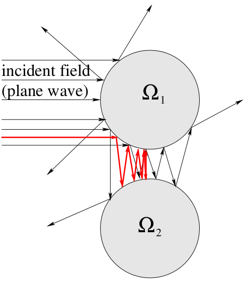
Scattering of an incoming plane wave

The mathematical formulation leads to an integral equation based on the Helmholtz kernel. Solving such an equation involves the discrete representation of the analytic operators and, if neccessary, the computation of a preconditioner. Both shall be performed using the H-matrix technique.

Problem Description

Let \(\Omega_i \in R^3, i = 1, \ldots, r\) be convex sets with smooth boundaries \(\Gamma_i = \partial \Omega_i\). Furthermore, let \(\nu = \nu_1, \nu_2, \ldots\) with \(1 \le \nu_i \le r\) be a sequence, such that \(\nu_i \ne \nu_{i+1}\) for all \(i\).

To compute: densities \(\eta_{\nu_i}\) on \(\Gamma_{\nu_i}\) defined by

\[ \eta_{\nu_i} - \mathcal{K}_{\nu_i} \eta_{\nu_i} = g_{\nu_i}, \]

with

\[ (\mathcal{K}_{\nu_i} \eta_{\nu_i})(x) := \int_{\Gamma_{\nu_i}} \frac{\partial G(x,y)}{\partial n(x)} \eta_{\nu_i}(y) dy, \quad x \in \Gamma_{\nu_i} \]

with \(G(x,y) = -\frac{1}{2\pi} \frac{e^{ik|x-y|}}{|x-y|}\), \(k > 0\) and with \(d \in R^3,\; |d| = 1,\)

\begin{eqnarray*} g_{\nu_i}(x) := \left\{ \begin{array}{ll} 2 \frac{\partial e^{ik \langle d,x \rangle }}{\partial n(x)}, & i = 1 \\ (\mathcal{K}_{\nu_{i-1}} \eta_{\nu_{i-1}})(x), \; x \in \Gamma_{\nu_i} & i > 1 \end{array} \right. \end{eqnarray*}

With a standard Galerkin discretisation using constant ansatz functions, one obtains the following matrices

\[ K^{\nu_i,\nu_i}_{ij} := \frac{1}{2\pi} \int_{\Gamma_{\nu_i}} \int_{\Gamma_{\nu_i}} e^{ik| x - y|} \frac{1-ik|x-y|}{|x-y|^3} \langle x-y, n( x ) \rangle dy dx \]

and

\[ K^{{\nu_i},{\nu_{i-1}}}_{ij} := \frac{1}{2\pi} \int_{\Gamma_{\nu_i}} \int_{\Gamma_{\nu_{i-1}}} e^{ik| x - y|} \frac{1-ik|x-y|}{|x-y|^3} \langle x-y, n( x ) \rangle dy dx \]

This leads to the following algorithm, which iterates between the surfaces \(v_i\):

  • build \(K^{1,1}, K^{2,2}, K^{2,1}\) and \(K^{1,2}\);
  • build initial right hand side \(b_{1,1} := g_1\);
  • for \(i = 1,\cdots\)
    • solve \((I - K^{1,1}) \eta_{i,1} = b_{i,1}\);
    • if \(\eta_{i,1} / \eta_{i-1,1}\) converged stop
    • \(b_{i,2} := K^{2,1} \eta_{i,1}\);
    • solve \((I - K^{2,2}) \eta_{i,2} = b_{i,2}\);
    • \(b_{i+1,1} := K^{1,2} \eta_{i,2}\);

Grid Definition

After the standard initialisation, which also imports the π–§π–«π–¨π–‘π—‰π—‹π—ˆ types for real and complex values,

#include <iostream>
#include <hlib.hh>
using namespace HLIB;
using namespace std;
using real_t = HLIB::real;
using complex_t = HLIB::complex;
int main ( int argc, char ** argv )
{
try
{
INIT();

the program begins with the definition of the grid for the surfaces \(\Gamma_1\) and \(\Gamma_2\). For this, the internal grid generation of π–§π–«π–¨π–‘π—‰π—‹π—ˆ is used to construct a spherical grid with radius 1 centered at \((0,0,0)\):

auto grid1 = make_grid( "sphere-5" );
grid1->scale( T3Point( 4, 4, 1 ) );

Here, "sphere-5" specifies the grid sphere with 5 refinement levels. The second command is optional. It deforms the sphere into a disc, which extends the scattering process.

Usually, a grid in π–§π–«π–¨π–‘π—‰π—‹π—ˆ will only define triangle normals. Since this leads to constant normal directions per triangle, the approximation of the Helmholtz DLP kernel is less accurate and may even lead to false results (think of scattering between parallel planes). Therefore, the grid file should contain vertex normals, which are used to interpolate normal directions for each point on the triangle, leading to a continuous normal direction on the surface.

If vertex normals are missing, the can be trivially added under the above assumptions since each vertex coordinate equals the corresponding normal direction. You may use add_vtx_normal of TGrid for this.

Since we need two surfaces, the process is repeated, but in addition, the second disc is shifted with respect to the z direction, such that both disc will have a positive distance:

auto grid2 = make_grid( "sphere-5" );
grid2->scale( T3Point( 4, 4, 1 ) );
grid2->translate( T3Point( 0, 0, 2.5 ) ); // distance 0.5

This leads to the following configuration:
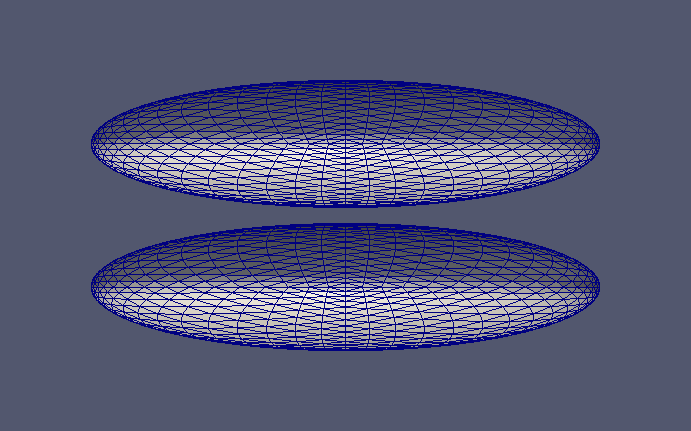
Grid with two discs

The construction of the grid ends with the definition of the corresponding function spaces. Here, we restrict ourselves to piecewise constant ansatz:

TConstFnSpace fnspace1( grid1.get() );
TConstFnSpace fnspace2( grid2.get() );

Matrix Construction

We need to construct the matrices \(K^{1,1}, K^{2,2}, K^{2,1}\) and \(K^{1,2}\). Due to definition of the grid, the matrices \(K^{1,1}\) and \(K^{2,2}\) are identical.

For the remaining matrices, cluster trees and block cluster trees are needed:

auto coord1 = fnspace1.build_coord();
auto coord2 = fnspace2.build_coord();
TAutoBSPPartStrat part_strat;
TBSPCTBuilder ct_builder( & part_strat );
auto ct1 = ct_builder.build( coord1.get() );
auto ct2 = ct_builder.build( coord2.get() );
TStdGeomAdmCond adm_cond( 2.0 );
TBCBuilder bct_builder;
auto bct11 = bct_builder.build( ct1.get(), ct1.get(), & adm_cond );
auto bct12 = bct_builder.build( ct1.get(), ct2.get(), & adm_cond );
auto bct21 = bct_builder.build( ct2.get(), ct1.get(), & adm_cond );

First, the matrix \(K^{1,1}\) shall be constructed. π–§π–«π–¨π–‘π—‰π—‹π—ˆ provides the class TAcousticScatterBF, which implements the kernel for \(G(x,y)\). Not defined so far is the wavenumber \(\kappa\), which should have a value of 6. Furthermore, ACA+ is used to compute low-rank approximations with a fixed block-wise accuracy of \(10^{-4}\).

using bf = TAcousticScatterBF< TConstFnSpace, TConstFnSpace >;
complex_t kappa( 4, 0 );
TTruncAcc acc = fixed_prec( 1e-4 );
unique_ptr< TMatrix > K11;
{
bf_t bf( kappa, & fnspace1, & fnspace1 );
TBFCoeffFn< bf_t > bf_coeff_fn( & bf );
TPermCoeffFn< complex_t > coeff_fn( & bf_coeff_fn, bct11->row_ct()->perm_i2e(), bct11->col_ct()->perm_i2e() );
TACAPlus< complex_t > lrapx( & coeff_fn );
TDenseMBuilder< complex_t > h_builder( & coeff_fn, & lrapx );
K11 = unique_ptr< TMatrix >( h_builder.build( bct11.get(), acc ) );
}
Remarks
Objects such as the bilinear form, the coefficient function or the low-rank approximation, which are specific for a single matrix are encapsulated in a block to prevent name clashes with the other matrices.

The actual operator in the above equation is \(I - K^{1,1}\). Here \(I\) is not the identity, but the mass matrix, as defined by the identity kernel:

using massbf_t = TMassBF< TConstFnSpace, TConstFnSpace >;
{
massbf_t bf( & fnspace1, & fnspace1 );
TBFCoeffFn< massbf_t > mass_coeff_fn( & bf );
TPermCoeffFn< real_t > coeff_fn( & mass_coeff_fn, bct11->row_ct()->perm_i2e(), bct11->col_ct()->perm_i2e() );
TACAPlus< real_t > lrapx( & coeff_fn );
TDenseMBuilder< real_t > h_builder( & coeff_fn, & lrapx );
M11 = unique_ptr< TMatrix >( h_builder.build( bct11.get(), acc ) );
M11->set_complex( true );
}

Finally, \(K^{1,1}\) is updated with the mass matrix:

add( 1.0, M11.get(), -1.0, K11.get(), acc );

The construction of \(K^{1,2}\) and \(K^{2,1}\) is similar to \(K^{1,1}\). Only the function spaces and block cluster trees will change.
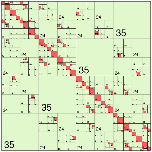
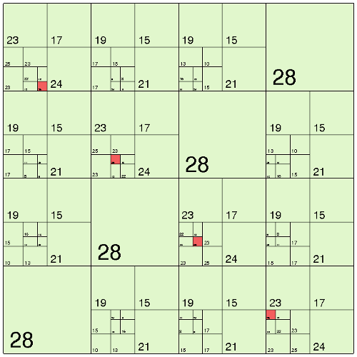
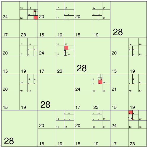
\(K^{1,1}\) \(K^{1,2}\) \(K^{2,1}\)

Please note, that \(K^{1,1}\) is more dense than the other two matrices. This is due to the positive distance between both discs. If this is increased (or if coarsening is applied), \(K^{1,2}\) and \(K^{2,1}\) may be represented by a single low-rank matrix.

Right-Hand Side

The initial right-hand side is defined by \(g_{\nu_i}\) above, where also the the incident field \(d\) is used:

\[ g_{\nu_i}(x) = 2 \frac{\partial e^{ik \langle d,x \rangle }}{\partial n(x)} \]

Under the above setting, this is equal to:

\[ g_{\nu_i}(x) = 2 i \kappa e^{ ik \langle d,x \rangle } \langle d, n \rangle \]

and is implemented in the following RHS function:

class TAcousticRHS : public TBEMFunction< complex_t >
{
private:
const T3Point _inc_dir; // incident direction
const complex_t _ikappa;
public:
TAcousticRHS ( const T3Point & inc_dir,
const complex_t kappa )
: _inc_dir( inc_dir )
, _ikappa( complex_t( 0, 1 ) * kappa )
{}
virtual complex_t
eval ( const T3Point & pos,
const T3Point & normal ) const
{
return real_t(2) * _ikappa * exp( _ikappa * dot( _inc_dir, pos ) ) * dot( _inc_dir, normal );
}
};

We use TQuadBEMRHS to compute the corresponding vector of the RHS using quadrature and afterwards reorder it for H-arithmetic:

TAcousticRHS rhsfn( T3Point( 1, 1, 0 ), kappa );
TQuadBEMRHS< TConstFnSpace, complex_t >
rhs_build( 4 );
auto rhs = rhs_build.build( & fnspace1, & rhsfn );
ct1->perm_e2i()->permute( rhs.get() );

The plane wave \(d\) is chosen to be \((1,1,0)\).

Acoustic Scattering Iteration

The scattering iteration involves to solves with \(K^{1,1}\) ( \(=K^{2,2}\)). This is accelerated using a preconditioner computed by and H-LU factorisation:

auto K11_copy = K11->copy();
auto K11_pre = factorise_inv( K11_copy.get(), acc );

We also need a vector to hold the current and the last approximation of the solution:

auto x = K11->col_vector();
auto x_old = K11->col_vector();
real_t old_ratio = real_t(1);

The variable old_ratio is needed to check convergence.

The iteration begins with solving \((I - K^{1,1}) \eta_{i,1} = b_{i,1}\), where \(b\) is the vector of the RHS:

for ( int it = 0; it < 100; ++it )
{
solve( K11.get(), x.get(), rhs.get(), K11_pre.get() );

Convergence is tested, if the ratio between the previous solution and the current solution is below some threshold. For this ratio is tested entry-wise, e.g. \(\eta_{i,1}^j / \eta_{i-1,1}^j\) for each \(j\). This is implemented in the function compare:

real_t
compare ( const TVector * x,
const TVector * x_old )
{
real_t vmax = 0.0;
size_t n = x->size();
for ( idx_t j = 0; j < idx_t(n); ++j )
{
const complex_t v = x->centry( j );
const complex_t v_old = x_old->centry( j );
vmax = std::max( vmax, abs( v / v_old ) );
}
return vmax;
}

If this ratio does no longer change, the iteration is stopped. The threshold in this example is \(10^{-4}\):

if ( it > 0 )
{
const real_t ratio = compare( x.get(), x_old.get() );
const real_t diff = ( it > 1 ? std::abs( ratio - old_ratio ) / std::abs( old_ratio ) : 1.0 );
old_ratio = ratio;
if ( diff < 1e-4 )
break;
}

In addition to this, the iteration shall stop if the solution \(\eta_{i,1}\) vanishes:

const real_t normx = x->norm2();
if ( x->norm2() < 1e-20 )
break;

Otherwise, the iteration continues with the scaling of the solution vector and the computation of the RHS for \(K^{2,2}\):

x->scale( real_t(1) / normx );
x_old->assign( real_t(1), x.get() );
mul_vec( real_t(-1), K12.get(), x.get(), real_t(0), rhs.get(), apply_normal );

Solving with \(K^{2,2}\) ( \(=K^{1,1}\)) and computing the RHS for the next iteration finished the loop and the program:

solve( K11.get(), x.get(), rhs.get(), K11_pre.get(), & solve_info );
mul_vec( real_t(-1), K21.get(), x.get(), real_t(0), rhs.get(), apply_normal );
}
DONE();
}
catch ( Error & e )
{
cout << e.to_string() << endl;
}
return 0;
}

Running the simulation will produce the following output for \(\eta_{i,1}\) and \(\eta_{i,2}\). Here, the entry-wise absolute values of the complex valued solution vectors are used for the visualisation (reload page to restart animation):

\(\eta_{i,1}\) \(\eta_{i,2}\)

The Plain Program

Remarks
Within the π–§π–«π–¨π–‘π—‰π—‹π—ˆ distribution you will find the full program with visualisation commands.
#include <iostream>
#include <hlib.hh>
using namespace HLIB;
using namespace std;
using real_t = HLIB::real;
using copmplex_t = HLIB::complex;
class TAcousticRHS : public TBEMFunction< complex_t >
{
private:
const T3Point _inc_dir; // incident direction
const complex_t _ikappa;
public:
TAcousticRHS ( const T3Point & inc_dir,
const complex_t kappa )
: _inc_dir( inc_dir )
, _ikappa( complex_t( 0, 1 ) * kappa )
{}
virtual complex_t
eval ( const T3Point & pos,
const T3Point & normal ) const
{
return real_t(2) * _ikappa * exp( _ikappa * dot( _inc_dir, pos ) ) * dot( _inc_dir, normal );
}
};
real_t
compare ( const TVector * x,
const TVector * x_old )
{
real_t vmax = 0.0;
size_t n = x->size();
for ( idx_t j = 0; j < idx_t(n); ++j )
{
const complex_t v = x->centry( j );
const complex_t v_old = x_old->centry( j );
vmax = std::max( vmax, abs( v / v_old ) );
}// for
return vmax;
}
int main ( int argc, char ** argv )
{
try
{
INIT();
auto grid1( read_grid( "sphere.tri" ) );
grid1->scale( T3Point( 4, 4, 1 ) );
auto grid2( read_grid( "sphere.tri" ) );
grid2->scale( T3Point( 4, 4, 1 ) );
grid2->translate( T3Point( 0, 0, 2.5 ) ); // distance 0.5
TConstFnSpace fnspace1( grid1.get() );
TConstFnSpace fnspace2( grid2.get() );
auto coord1 = fnspace1.build_coord();
auto coord2 = fnspace2.build_coord();
TAutoBSPPartStrat part_strat;
TBSPCTBuilder ct_builder( & part_strat );
auto ct1 = ct_builder.build( coord1.get() );
auto ct2 = ct_builder.build( coord2.get() );
TStdGeomAdmCond adm_cond( 2.0 );
TBCBuilder bct_builder;
auto bct11 = bct_builder.build( ct1.get(), ct1.get(), & adm_cond );
auto bct12 = bct_builder.build( ct1.get(), ct2.get(), & adm_cond );
auto bct21 = bct_builder.build( ct2.get(), ct1.get(), & adm_cond );
complex_t kappa( 6, 0 );
TTruncAcc acc = fixed_prec( 1e-4 );
unique_ptr< TMatrix > K11;
{
bf_t bf( kappa, & fnspace1, & fnspace1 );
TBFCoeffFn< bf_t > bf_coeff_fn( & bf );
TPermCoeffFn< complex_t > coeff_fn( & bf_coeff_fn, bct11->row_ct()->perm_i2e(), bct11->col_ct()->perm_i2e() );
TACAPlus< complex_t > lrapx( & coeff_fn );
TDenseMBuilder< complex_t > h_builder( & coeff_fn, & lrapx );
K11 = h_builder.build( bct11.get(), acc );
}
unique_ptr< TMatrix > M11;
{
massbf_t bf( & fnspace1, & fnspace1 );
TBFCoeffFn< massbf_t > mass_coeff_fn( & bf );
TPermCoeffFn< real_t > coeff_fn( & mass_coeff_fn, bct11->row_ct()->perm_i2e(), bct11->col_ct()->perm_i2e() );
TACAPlus< real_t > lrapx( & coeff_fn );
TDenseMBuilder< real_t > h_builder( & coeff_fn, & lrapx );
M11 = h_builder.build( bct11.get(), acc );
M11->set_complex( true );
}
add( 1.0, M11.get(), -1.0, K11.get(), acc );
unique_ptr< TMatrix > K12;
{
bf_t bf( kappa, & fnspace1, & fnspace2 );
TBFCoeffFn< bf_t > bf_coeff_fn( & bf );
TPermCoeffFn< complex_t > coeff_fn( & bf_coeff_fn, bct12->row_ct()->perm_i2e(), bct12->col_ct()->perm_i2e() );
TACAPlus< complex_t > lrapx( & coeff_fn );
TDenseMBuilder< complex_t > h_builder( & coeff_fn, & lrapx );
K12 = h_builder.build( bct12.get(), acc );
}
unique_ptr< TMatrix > K21;
{
bf_t bf( kappa, & fnspace2, & fnspace1 );
TBFCoeffFn< bf_t > bf_coeff_fn( & bf );
TPermCoeffFn< complex_t > coeff_fn( & bf_coeff_fn, bct21->row_ct()->perm_i2e(), bct21->col_ct()->perm_i2e() );
TACAPlus< complex_t > lrapx( & coeff_fn );
TDenseMBuilder< complex_t > h_builder( & coeff_fn, & lrapx );
K21 = h_builder.build( bct21.get(), acc );
}
TAcousticRHS rhsfn( T3Point( 1, 1, 0 ), kappa );
TQuadBEMRHS< TConstFnSpace, complex_t >
rhs_build( 4 );
auto rhs = rhs_build.build( & fnspace1, & rhsfn );
ct1->perm_e2i()->permute( rhs.get() );
auto K11_copy = K11->copy();
auto K11_pre = factorise_inv( K11_copy.get(), acc );
auto x = K11->col_vector();
auto x_old = K11->col_vector();
real_t old_ratio = real_t(1);
for ( int it = 0; it < 100; ++it )
{
solve( K11.get(), x.get(), rhs.get(), K11_pre.get() );
if ( it > 0 )
{
const real_t ratio = compare( x.get(), x_old.get() );
const real_t diff = ( it > 1 ? std::abs( ratio - old_ratio ) / std::abs( old_ratio ) : 1.0 );
old_ratio = ratio;
if ( diff < 1e-4 )
break;
}
const real_t normx = x->norm2();
if ( x->norm2() < 1e-20 )
break;
x->scale( real_t(1) / normx );
x_old->assign( real_t(1), x.get() );
mul_vec( real_t(-1), K12.get(), x.get(), real_t(0), rhs.get(), apply_normal );
solve( K11.get(), x.get(), rhs.get(), K11_pre.get() );
mul_vec( real_t(-1), K21.get(), x.get(), real_t(0), rhs.get(), apply_normal );
}
DONE();
}
catch ( Error & e )
{
cout << e.to_string() << endl;
}
return 0;
}
HLIB::TMassBF
bilinear form for mass matrix
Definition: TMassBF.hh:25
HLIB::BLAS::dot
enable_if_res< is_vector< T1 >::value &&is_vector< T2 >::value &&is_same_type< typename T1::value_t, typename T2::value_t >::value, typename T1::value_t >::result dot(const T1 &x, const T2 &y)
compute <x,y> = x^H Β· y
Definition: Algebra.hh:283
HLIB::TBCBuilder
Recursively build block cluster tree with supplied admissibility condition.
Definition: TBCBuilder.hh:27
HLIB::TBSPCTBuilder
Base class for all cluster tree constructors based on BSP.
Definition: TBSPCTBuilder.hh:161
HLIB::TBCBuilder::build
virtual std::unique_ptr< TBlockClusterTree > build(const TClusterTree *rowct, const TClusterTree *colct, const TAdmCondition *ac) const
HLIB::TACAPlus
Implements ACA+, which corrects some of the deficits of the original ACA algorithm.
Definition: TLowRankApx.hh:474
HLIB::TAcousticScatterBF
Bilinear form for acoustic scattering.
Definition: TAcousticBF.hh:30
HLIB::read_grid
std::unique_ptr< TGrid > read_grid(const std::string &filename)
Read grid from file with automatic file format detection.
HLIB::TAutoBSPPartStrat
Automatic choice of best partitioning strategy.
Definition: TBSPPartStrat.hh:174
HLIB::TVector::size
virtual size_t size() const =0
return size of vector
HLIB::eval
void eval(const TMatrix *A, TVector *v, const matop_t op, const eval_option_t &options)
evaluate LΒ·UΒ·x=y with lower triangular L and upper triangular U
HLIB::mul_vec
void mul_vec(const TProcSet &ps, const real alpha, const TMatrix *A, const TVector *x, const real beta, TVector *y, const matop_t op)
compute y ≔ Ξ±Β·AΒ·x + Ξ²Β·y on (possibly) distributed matrix A on all processors in ps
HLIB::TMatrix::copy
virtual auto copy() const -> std::unique_ptr< TMatrix >
return copy of matrix
HLIB::TPermCoeffFn
Eval coefficient function with reordered indices, e.g. change internal to external ordering.
Definition: TCoeffFn.hh:138
HLIB::add
void add(const T_value alpha, const TMatrix *A, const T_value beta, TMatrix *C, const TTruncAcc &acc)
C ≔ Ξ±Β·A + Ξ²Β·C.
HLIB::TMatrix::col_vector
virtual auto col_vector() const -> std::unique_ptr< TVector >
return appropriate column vector object for matrix
Definition: TMatrix.hh:610
HLIB::TMatrix::set_complex
void set_complex(const bool b, const bool force=false)
Definition: TMatrix.hh:290
HLIB::TBFCoeffFn
Provide matrix coefficients defined by bilinear forms.
Definition: TBFCoeffFn.hh:27
HLIB::TTruncAcc
Defines accuracy for truncation of low rank blocks.
Definition: TTruncAcc.hh:33
HLIB::TStdGeomAdmCond
Standard admissibility for FEM/BEM applications normal : adm iff min( diam(Ο„), diam(Οƒ) ) ≀ Ξ·Β·dist(Ο„,...
Definition: TGeomAdmCond.hh:28
HLIB::BLAS::solve
enable_if< is_matrix< T1 >::value &&is_vector< T2 >::value &&is_same_type< typename T1::value_t, typename T2::value_t >::value >::result solve(T1 &A, T2 &b)
solve AΒ·x = b with known A and b; x overwrites b (A is overwritten upon exit!)
Definition: Algebra.hh:997
HLIB::TVector::assign
virtual void assign(const real, const TVector *)
this ≔ f Β· vector
Definition: TVector.hh:167
HLIB::factorise_inv
std::unique_ptr< TFacInvMatrix > factorise_inv(TMatrix *A, const TTruncAcc &acc, const fac_options_t &options=fac_options_t())
compute factorisation of A and return inverse operator
HLIB::TVector::centry
virtual const complex centry(const idx_t i) const
return i'th entry
HLIB::TDenseMatBuilder
Creates matrices by computing low rank approximations of dense sub matrices, e.g. via ACA or SVD.
Definition: TMatBuilder.hh:310
HLIB::TVector
Base class for all vectors defining basic interface.
Definition: TVector.hh:33
HLIB::TVector::scale
virtual void scale(const real)
scale vector by constant factor
Definition: TVector.hh:163
HLIB::TVector::norm2
virtual real norm2() const
return euclidean norm
Definition: TVector.hh:178